Suppose we have followed our methodology, and just made some modification of our previously running program. Unfortunately, after the change the program stops working. What do we do next to find the problem and to correct it? We first have to understand what types of errors can occur in an ECLiPSe program.
We can distinguish five types of failure, each with its own set of causes and possible remedies.
Run-time errors occur if we call a built-in predicate with a wrong argument pattern. This will usually either be a type mismatch, i.e. using a number where an atom is expected, or an instantiation problem, i.e. passing a variable where a ground value was expected or vice versa. In this case the ECLiPSe system prints out the offending call together with an error message indicating the problem. If we are lucky, we can identify the problem immediately, otherwise we may have to look up the documentation of the built-in to understand the problem.
In the following example bug0, we have called the predicate open/3 with an incorrect first argument.
:-export(bug0/0).
bug0:-
        open(1,read,S), % wrong
        read(S,X),
        writeln(X),
        close(S).
When we run the query bug0, the ECLiPSe system prints out the message:
type error in open(1, read, S)
In general run-time errors are quite simple to locate and to fix. But the system does not indicate which particular call of a built-in is to blame. We may need to use the tracer to find out which of dozens of calls to the predicate is/2 for example may have caused a particular problem. There are several things that may help to avoid the tedious tracing.
These errors occur when we hit some limit of the run-time system, typically exceeding available memory. An example is the run-away recursion in the program bug1 below:
:-export(bug1/0).
bug1:-
        lp(X),  % wrong
        writeln(X).

lp([_H|T]):-
        lp(T).
lp([]).
After some seconds, the system returns an error message of the form:
*** Overflow of the local/control stack!
You can use the "-l kBytes" (LOCALSIZE) option to have a larger stack.
Peak sizes were: local stack 13184 kbytes, control stack 117888 kbytes
Typical error sources are passing free variables to a recursion, where the terminating clause is not executed first or the use of an infinite data structure.
Probably the most common error symptom is a failure of the application. Instead of producing an answer, the system returns ’no’. This is caused by:
The best way of finding failures is by code inspection, helped by logging messages which indicate the general area of the failure. If this turns out to be too complex, we may have to use the tracer.
More rare is the situation where a “wrong” answer is returned. This means that the program computes a result, which we do not accept as an answer. The cause of the problem typically lies in a mismatch of the intended behaviour of the program (what we think it is doing) and the actual behaviour.
In a constraint problem we then have to identify which constraint(s) should eliminate this answer and why that didn’t happen. There are two typical scenarios.
We can often distinguish these problems by re-stating the constraint a second time after the wrong answer has been found.
If the constraint still accepts the solution, then we can assume that it simply does not exclude this solution. We will have to reconsider the declarative definition of the constraint to reject this wrong answer.
If the program fails when the constraint is re-stated, then we have a problem with the dynamic execution of the constraints in the constraint solver. That normally is a much more difficult problem to solve, and may involve the constraint engine itself.
Probably the most complex problem is a missing answer, i.e. the program produces correct answers, but not all of them. This assumes that we know this missing answer, or we know how many answers there should be to a particular problem and we get a different count when we try to generate them all. In the first case we can try to instantiate our problem variables with the missing answer before stating the constraints and then check where this solution is rejected.
This type of problem often occurs when we develop our own constraints and have made a mistake in one of the propagation rules. It should not occur if we use a pre-defined constraint solver.
A very simple debugging technique is the logging of certain predicate calls as they occur in the program.
:-export(bug2/0).

bug2:-
        ...
        generate_term(Term),
        analyze_term(Term,Result),
        ...
Suppose we assume that the predicate analyze_term is responsible for a problem. We can then simply add a writeln call before and/or after the predicate call to print out the suspected predicate. The output before that call should show all input arguments, the output after the call should also show the output results.
:-export(bug2/0).

bug2:-
        ...
        generate_term(Term),
        writeln(analyze_term(Term,Result)),
        analyze_term(Term,Result),
        writeln(analyze_term(Term,Result)),
        ...
Used sparingly for suspected problems, this technique can avoid the use of the debugger and at the same time give a clear indication of the problem. The ECLiPSe system will normally restrict the output of a term to a certain complexity, so that long lists are not printed completely. This can be influenced by the print_depth flag of set_flag.
Such messages can be written to the log_output stream (or a user-defined stream) which can be later be discarded by
set_stream(log_output,null)
or which can be directed to a log file. This can be useful in “live” code, in order to capture information about problems in failure cases.
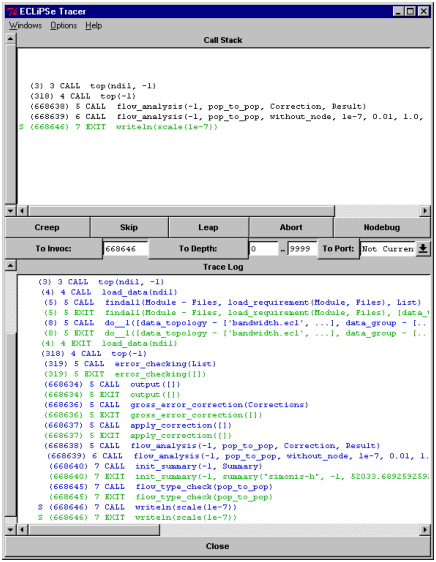
Ideally, we can figure out all problems without running the application in the debugger. But at some point we may need to understand what the system is doing in more detail. We can then start the ECLiPSe tracer tool from the Tools menu. Figure 7.1 shows a typical output. In the top window we see the current stack of predicate calls, in the bottom we see a history of the program execution.
The three buttons Creep, Skip, Leap show the main commands of the tracer. The creep operation single-steps to the next statement in the program. The skip operation executes the current query and stops again when that query either succeeds or fails. The leap operation continues execution until it reaches a spy point, a predicate call for which we have indicated some interest before.
A normal debugging session consists of a sequence of leap, skip and creep operations to reach an interesting part of the program and then a more detailed step-by step analysis of what is happening. It is pointless and very time consuming to single-step through a part of the program that we have already checked, but we have to be careful not to skip over the interesting part of the program.
In a large program, it may be difficult to leap directly to the interesting part of the program. But we may have to repeat this operation several times, if we repeatedly leap/skip over an interesting statement. We can use the invocation number of a statement to jump to this exact place in the execution again. The invocation number is printed in parentheses at the beginning of each trace line. By re-starting the debugger, copying this number into the text field to the right of the button To Invoc: and then pressing this button we can directly jump to this location.
Unfortunately, jumping to an invocation number can be quite slow in a large program. The debugger has to scan each statement to check its invocation number. It can be faster (but more tedious) to use skip and leap commands to reach a program point1.